Information note n°31a

Analysis of the observations of contacts

The on-line calculation of the AU in real time :

P. Rocher, J.-E. Arlot, September 20, 2004.

How can we calculate the value of the AU from a measure of time?

Before describing the methods that we used, let’s come back to the nature of the measurement performed.

Description of the experiment.

We received a lot of e-mails showing that most of the observers did not understand the problem and think that measuring the astronomical unit (AU) through the observation of the contacts is the same than measuring the length of an object using a ruler. Then, they think that all the measures are equivalent and that the final result is the average of all the measurements. In reality, it is not like this.

The measure of the AU through the observation of contacts is not a measure of distance, but a measure of time, this time being not the same for all the observers. In fact, the phenomenon that we observe comes from the parallax existing between the direction of the contact from the centre of the Earth (theoretically calculated) and the direction of the contact from the observing site. The observed timing will be used to calculate the corresponding AU.

More, in our experiment, we do not choose the observed parallaxes since the observers do not move towards a specific optimum sites (where the parallax is maximum) as did the astronomers of the past centuries and the distribution of the observers on Earth is random (in fact concentrated in Europe…).

So, for a calculation in real time of the AU, it is not possible to use the Delisle’s method which associates two sites well situated on Earth. We should calculate the AU by comparing each observation to the theoretical value: which has to be the value of the ua so that the difference between the moments of contact observed and calculated are smallest possible?

 However, another problem emerges: the convergence of the algorithm. An observation leading to put the Sun at the infinite will corrupte the average. Since we do not know in advance the accuracy of the observation, it is not possible to choose a criterion allowing to reject “bad” observations. Then, we had to build an algorithm containing a strong constraint avoiding the algorithm to diverge.

Our algorithm of calculation of the AU is as follows :

-         arriving of an observation of a contact, calculation of the corresponding AU

-         arriving of a second observation, calculation of the corresponding AU and then, averaging with the preceding calculated AU

-         and so on, the nth observation providing a calculated AU which will be averaged with the (n-1)th preceding calculated AU.

Note that it is not possible to modify the criteria of rejection of observation during the run starting June 8 : all the observations should be accepted (within 30 minutes of time) and the « bad » observations may not disturb the calculations.

What are we measuring and what are we calculating ?

The problem that we solve is the calculation of the diurnal parallax of a point of contact as seen from a given observing site by measuring the shift in time between the observed and the theoretical timing of the contact.

The figure below explains the geometry of the problem :

 

Figure 1 : The diurnal parallax

On this figure, O is the observer, OX is the line of sight of the direction of the contact and the line XC joins the point of contact X on the limb of the Sun to the centre C of the Earth.

The predictions are made using the value of the solar parallax p₀=8,794142", thus using a value of the AU perfectly known nowadays, AU = 149597870 km. The prediction t_c of the time of the contact consists in finding, knowing the size of the triangle XOC thanks to the knowledge of the AU, at what time will occur the contact. Mathematically, we have a relationship R (a function) which, for any observing site, provides a value of t_c from the value of the AU. This function depends on numerous physical parameters such as the diameters of the Sun and Venus in km, the position of the observer, the equatorial radius of the Earth and its flatness, and the position of the centres of Venus and the Sun at any time..

The calculation of the AU from the observation of the timing of a contact consists in the inverse operation (in mathematics, the reciprocal function R^-1) : what should be the value of the AU in km so that the calculated time of the contact t_c (using the relationship R) be the same than the observed value ?

It is possible theoretically, to calculate for each observation of contact received, a corresponding value of the AU.

How these individual calculated AU will be used ?

The only possible calculation to be made in real time when receiving the observations is the averaging of the calculated AU of individual observations and to calculate a statistical parameter, the experimental standard deviation.

So we must be aware of the difference between the measure made – a timing – and the corresponding calculation of a AU. We did not measure directly the AU (as with a ruler), but the AU is the result of a calculation based upon the measure of a time.

 

An important note in order to understand the next steps :

What is a « good » measure ?

Intuitively, a « good » measure is a measure as close to the reality as possible and which did not send the Sun at the infinite ! The experience of the past centuries let us think that an error of one minute of time on a timing of a contact may be commonplace among the observers. However, as we are now at the XXIst century (use of GPS, recording of CCD images, use of good optics, inexperience of the observers, …) things have changed but, before the observations of June 8, we did not know what will be the real mean error on the measurements. This will not be a help for the real time calculation.

More, suppose that we get « good » measures : may we say now that such a good measure of the timing of a contact will lead to a good value of the AU ?

Unfortunately the answer is not always : it depends on the contact involved and on the site of observation.

We can explain this in two ways :

·        First from geometrical considerations. On the figure 1, it is evident that the form of the triangle XOC depends on the position of the observer O. If the observer is in Y, the angle OXC is zero : the triangle is completely flat an dit is impossible to make any measurement (the diurnal parallax is zero and the calculation does not depend on the value of the AU). Contrarily, if the observer is in Z, the angle OXC is at his maximum (the angle XOC is 90°), the diurnal parallax is maximum. Attention, we did not measure the diurnal parallax but the effect of the diurnal parallax on the calculation of the times of contacts. The form of the triangle characterizes the geometry of the problem but the effect of the diurnal parallax may be zero even if the diurnal parallax is maximum. Thus, for a given geometrical contact, all the sites on Earth defined by the intersection of the cone of shadow (or penumbra depending on the contact) with the terrestrial ellipsoid will see the contact at the same time as an observer situated at the center of the Earth. So, more we are close to these sites, more the effect of the diurnal parallax is small.

A good site of observation must verify two criteria : to have a diurnal parallax as large as possible and to be as far as possible from the intersection of the cone of shadow (or penumbra) with the terrestrial ellipsoid. The worst site of observation on Earth for this method is the point of this line of intersection which have a diurnal parallax being zero, i.e. the point of contact being at the zenith. For each contact, only one site exits corresponding to that criterion. In conclusion a good site of observation must be far from this line of intersection and must observe the contact when the Sun i slow above the horizon.

• Second, from the linear approached formula providing the variation of the parallax from the variation of the time shift (see information sheet n°4b).

 

For each contact, the coefficients A, B, C and the value dD/dt are fixed.

For example, for the first internal contact, we have :

A = 2,1970, B = 0,2237, C = 1,1206, dD/dt = –2,9394"/min.

Let’s have 

The variation of the parallax for a given shift (t_o-t_c) is the quotient of 2,9394 per X. However, this coefficient is function of the coordinates of the observer : it tends towards zero when the observer approaches the points of the Earth whose geographical coordinates are solution of the equation X=0.

Thus for the same variation of observation in time, one can obtain very important differences on the variation of the parallax and thus of the AU. This one becomes even infinite when X is null, even with a very good observation!

We also can indicate the geometrical difference between direct calculation and linearized calculation. The X=0 equation has, as a solution, the intersection of a plan passing by the centre of the Earth, with the terrestrial ellipsoid; the real solution is the intersection of a cone with the terrestrial ellipsoid, the linearization thus replaces the cone by a tangent plan to a cone passing by the centre of the Earth.

 

The solution of the « constrained » system.

We saw above that it was possible, theoretically, to calculate a value of the AU for any observed timing t_o of a contact made from any site of observation. We saw, then, that in fact, it was impossible for timings made in some sites, timings leading to an infinite value for the AU. For timings away from the right value of several minutes of time (which could be commonplace after the experience of the past centuries), the algorithm for the calculation of the reciprocal function did not converge..

Since we would like to take into account all the received observations in order to make an averaging as the observations arrived. In order to be sure to succeed in the calculation, we solved a system slightly different in which we put a constraint in order to avoid the calculated value of the AU to become infinite. Of course, we did not constrain totally the system (i.e. we did not impose the value of the AU) but we forced the triangle XOC to remain a finite triangle (i.e. to prevent the Sun and Venus to leave ad infinitum). For that, in the calculation of the reciprocal function providing the value of the AU depending on the observed timing, we multiplied the vectors Earth – Venus and Earth – Sun by the ratio CAU/EAU, where CAU is the calculated AU and EAU the estimated AU. Such a system converges towards the value of the AU as the system without such a constraint but it has the advantage of having a solution for all the possible values permitted during the acquisition of the data (no more than 30 minutes error on the timings). However, the convergence of the calculation needed also that the observer did not observe at the zenith (the result being meaningless), that was, fortunately, not the case.

Normaly, if the observations are realistic, i.e. if the observers send the timings they really measure, the average of AU of the constrained system is the same than with the not constrained system in which the too bad observations have been rejected. This is not true if the observers entered non realistic timings just to test the algorithm (to try to make the calculations divergent !). Such entries occurred after June 18, the database still accepting new data and the average of the calculated AU was degraded.

So we may say that the effects of the constrained system was in fact to improve artificially the quality of the observations for the calculation of the AU but as in the non constrained method, the site of observation was very important and it is not possible to compare results from one site to another either in the constrained system or in the non constrained..

In conclusion, we provided to the observers in real time their individual results, the error on which appearing to be better than with the non constrained system (but comparable between themselves, from an observer to another) since the average on the AU was realistic. We could have provided the difference between the observed timing and the true one to the observers but since it was still possible to enter a new observation certain observers could have been tempted to cheat !

You will find below the plot of the evolution of the average of the AU (for the four contacts) as we received data (in green) and the evolution of the dispersion (experimental root mean square of the residuals s) in blue. We stop on June 18, date after what false data were enterd for test by some registered observers.

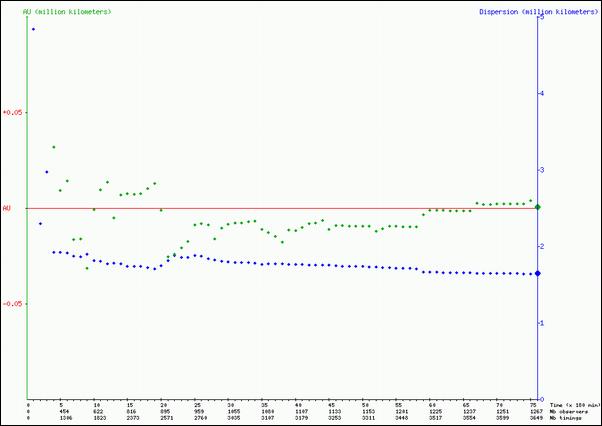
Evolution of the average of AU and dispersion of the data until June 18.

 

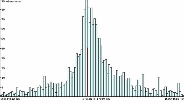
Distribution of the AU calculated using all the database.

You will find below the final results obtained with the constrained system using all the observations until an error of about 30 minutes of time :

 

Contact	Number of observations	AU in km	Shift to true AU in km	Experimental dispersion	Parallax
T1	722	149908018	-310148	2062405	8,775936"
T2	1139	149076728	521142	4878994	8,824890"
T3	1336	149438938	158932	1409362	8,803500"
T4	1170	149840793	-242923	4620163	8,779890"
All	4367	149529684	68186	3638485	8,798158"
Average (T1+T2+T3+T4)/4		149566119	31751		8,796015"

Table 1

The distribution of the values of the AU from the whole database used for the averaging shows that it follows a normal law an dis gaussian. If the false value are rejected, the distribution is better. The supposition of a distribution according to a normal law is  justified ; then the average of the calculated AU is a good estimator of the AU an dit is possible to calculate the dispersion by dividing the experimental dispersion by the square root of the number of observations.

We will find finally, using all the observations of all the contacts :

AU = 149 529 684 km +/- 55 059km.

The shift to the « true » AU being 68 186 km.

Let us note that during our real time calculation, we published the average of the calculated AU for each contact and not the general average of all the observations. That involved a curious result at the beginning of experiment: an observer entered a value of the first or second contact for a contact which had not taken place yet (the third or the fourth) ; that gave a result, single and false for this contact, which entered in our average. Afterwards, this bad result was averaged progressively as the data arrived concerning this contact and its influence disappeared rapidly.

We will see in the information note n°31b the not constrained system provides results similar to the ones of the constrained system when using only the values of the intervals of 16s and 8s around the predicted values of the contacts.