Information note n°31b

Analysis of the observations of contacts

Calculation of the AU using the whole set of data :

P. Rocher, J.-E. Arlot, September 18, 2004.

Introduction.

We are now after June 8 and we have received all the observations of contacts. We may calculate the AU using a not constrained system or using the Delisle’s method using only some selected observations. For that purpose, we must find a criterion to select the “good” observations of contacts. In a first step we will suppose that the « good » observations are the ones near the predictions that we made. We will verify afterwards that this hypothesis is justified.

Then, we will select several sets of observations and we will calculate the AU using the not constrained method. We will also made the calculation after weighting the observations depending on the site of observation that should lead to a more realistic value of the AU. At last we will apply the Delisle’s method on our best set of data in order to see if it is applicable even if the observers were not organized as during the past centuries.

The calculation of the AU with the whole database of contacts

First, we have to be sure that the theoretical value of the parallax (or the AU) entered in the calculation of prediction of the contacts is good, compared to the experience that we are performing (i.e. the observation of the contacts for the determination of the AU).

How to do that ?

If this theoretical value is good, the average of the AU that we are calculating thanks toi the observations of contacts must converge as we decrease the interval of time around the predicted value in which we keep the sample of observations that we keep.

More explanations: we select all the observations being made at most at 30 seconds of time, for example, from the prediction and we make the average of the AU calculated with these observation. Then, we decrease the interval (15s, 8s, 4s) and we make the average of the calculated AU for each sample corresponding to each interval. If our initial theoretical value of the AU used for the prediction is good, the succession of averages converges towards our initial value. At the same time, the number of observed contacts late referred to the prediction will approach the number of contacts in advance and the average of these variations will tend towards zero insofar as the distribution of errors is Gaussian. This will be shown by the analysis of the data that we received.

Below, the results obtained with the whole data base as it was on July 14, 2004.

Characteristics of the data base :

Number of registered observers having sent observations : 1501.

Number of registered observers having observed the first contact : 722.

Number of registered observers having observed the second contact : 1139.

Number of registered observers having observed the third contact :1336.

Number of registered observers having observed the fourth contact :1170.

Number of registered observers having measured the external duration : 639.

Number of registered observers having measure the internal duration: 1014.

Number of registered observers having measured the four contacts: 616.

Total number of observations : 4367.

In the table below, we provide successively : the size of the interval 2DT around the predicted values of the contacts, the number of observations corresponding to this criterion, the average of the calculated AU solving the not constrained system with these observations, the shift to the real value of the AU and the value of the corresponding parallax.

Size of the interval	Number of observations	Average of the calculated AU	Shift to the true AU	Corresponding parallax
60s	2459	148511434 km	1086436 km	8,858482"
30s	1719	148789697 km	808172 km	8,841915"
16s	1066	149421803 km	176067 km	8,804510"
8s	583	149608708 km	-10838 km	8,793511"

Table 1

This analysis of the observations proves that the experiment confirms that the initial value of the parallax (or AU) used for the predictions is correct and mainly, this confirms the quality of the predictions made with this value. This result comes from the fact that the data base contains many observations (1066) close to the prediction (in the interval of 8s).

From now on, the definition of a “good” observation is an observation being close to the predictions since our predictions are close to the reality. We have now an objective criterion for the selection of observations in the data base.

This result has been obtained by analysis of observations from 1501 observers representing 4367 contacts. It was not possible to get such a result in real time on June 8 since we did not know in advance what will be the “good” observations and if the errors will follow a normal law (Gaussian distribution).

Results for an interval of 16s for each contact :

The following tables provide successively for each contact and for all contacts together the number of observations corresponding to the interval of 16s, the number of observations in advance referred to the prediction and the number of observations late, then the average of the calculated values of the AU using these observations, the shift to the true value of the AU, the standard deviation and the parallax corresponding to the calculated AU.

Contact	Number of observations	Number of observations in advance from T_c	Number of observations late from T_c	Average AU in km	Shift to the true value in km	Standard deviation in km	Parallax in arcsec
T₁	104	49	55	149443844	154026	186773	8.803212"
T₂	262	128	134	149590268	7602	108359	8.794595"
T₃	421	187	234	149226725	371145	324822	8.816020"
T₄	279	130	149	149549752	48118	70599	8.796978"
All	1066			149421803	176067	252081	8.804510"

Table 2.

So, using all the observations within 8s to the prediction (interval of 16 sec), we get the following result: AU = 149421803 km +/- 252081 km

For the calculation of these values, we calculate the average of the (the calculated AU for each observation).

Then we calculate the experimental variance and the experimental standard deviation of these measures of the AU.

At last, supposing that is a random variable following a normal law (Gaussian distribution of the errors), i.e. that the observations are without biases, then is a good estimator of the AU and the standard deviation on this estimator is given by :

Be careful to do not confuse the experimental standard deviation s on the measures which is independent of the law of distribution of the observations and the standard deviation on the estimator which depends on the law of distribution of the observations

We may remark that we have, as envisaged, a rather good distribution of the observations before and after the predicted values. We may remark also that the value of the calculated AU using the third contacts is the worst with the largest standard deviation. This comes from observations mainly made when the Sun is near the zenith for the observers (with a small diurnal parallax).

Tableau 3 is identical to table 2, but for the observations corresponding to an interval of 8s.

Contact2Dt = 8s	Number of obser-vations	Number of observations in advance on T_c	Number of observations late on T_c	Average of the AU in km	Shift to the true AU in km	Standard deviation of the AU in km	Parallax in arcsec
T₁	60	23	37	149725155	-127285	131387	8.786672"
T₂	148	67	81	149618152	-20282	69271	8.792956"
T₃	225	102	123	149267460	330410	217813	8.813614"
T₄	150	76	74	150064685	-466815	55667	8.766792"
All	583			149608708	-10838	11835	8.793511"

Table 3

So, using all the observations within 4s to the prediction (interval of 8 sec), we get the following result: AU = 149608708 km +/- 11835 km

We may remark that for each contact taken separately, the results tend to be degraded ; the values of the AU obtained using the contacts T₃ and T₄ show standard deviations smaller than the shift to the true value of the AU: the distribution of the errors may not be Gaussian. Contrarily, the result using all contacts is better.

Why the results from the third contact are so bad ? Quite simply because very many places of observations have a weak diurnal parallax at the time of the third contact (Sun too high above the horizon) and because they are too close to the intersection of the shadow cone at the time of the third geocentric contact with the terrestrial ellipsoid. One can visualize that on a map by plotting on the terrestrial sphere the four curves intersections of the cones of shadow and penumbra with the terrestrial ellipsoid at the moments of the geocentric contacts.

The closer one group of observers is to one of these curves, the more the effects of the diurnal parallax for the corresponding contact will be small and more the dispersion of the measurements is likely to be large if it is not compensated by very good measures of the contacts. Moreover the observation of the moments of interior contacts T3 is a little more difficult than that of the external contacts T4 because of the black drop. Thus the contacts T3 and T4 should be easier to observe than the contacts T1 and T2 since the majority of the observers observed them high in the sky, but, although better (225 observations retained here for T3 against 148 for T2) these observations give worse results, precisely because the Sun is close to the zenith.

Weighted average.

In the preceding calculation, we were satisfied to make the average of all the calculated values of the astronomical unit and we allotted the same weight to each result. However it is known that the errors of observation, for a contact given, from a place badly located can generate important variations in the results. Thus a random error of a few seconds on the measurement of a contact can have effects more or less strong on the value of the calculated AU.

We thus will try to weight these results by giving a weight to each observation, this weight will be all the more weak as the place is badly located for a contact considered.

If it is supposed that the observations are made without skew with a random error t. then the standard deviations on the parallax or the astronomical unit can be estimated, for each observation, by :

where t_c is the instant of the topocentric contact calculated and t_G is the instant of the geocentric contact.

One can take as weight of each observation :

Then the weighted averages of the astronomical unit and the parallax are calculated starting from the individual values a(k) ou p(k) calculated for each observation k using the two folowing relationships :

and the standard deviations on the weighted averages are given by :

Here results obtained on the sample of the 1066 observations of the contacts included in the interval 16 seconds around the predicted values and if it is supposed that the random error on each observation is of +/- 5s. This table is to be compared with table 2.

Contact	Number of observations	Weighted average AU in km	Shift to the true AU in km	Standard deviation in km	Parallax in arcsec	Standard deviation on the parallax
T₁	104	149491052	106818	194889	8,800432"	0,011457"
T₂	262	149564790	33080	114908	8,796093"	0,006755"
T₃	421	149424892	172978	231528	8,804328"	0,013610"
T₄	279	149312924	284946	285616	8,810931"	0,016790"
All	1066	149507347	90523	86718	8,799473"	0,005098"

Table 4

If the assumption is made that the random error on each observation is of +/- 10s, then the following results are obtained :

Contact	Number of observations	Weighted average AU in km	Shift to the true AU in km	Standard deviation in km	Parallax in arcsec	Standard deviation on the parallax e
T₁	104	149491052	106818	389778	8,800432"	0.022913"
T₂	262	149564790	33080	229816	8,796093"	0.013510"
T₃	421	149424892	172978	463056	8,804328"	0.027221"
T₄	276	149312924	284946	571233	8,810931"	0.033580"
All	1066	149507347	90523	173437	8,799473"	0.010196"

Table 4 bis

It is noted that the weighted averages do not change but that the standard deviations on these averages doubled, from where importance of the estimate of the error of measurement in the observations of times of contact.

Broadly the weighted average gives better results since the badly situated sites of observation have less weight. It is not true for the contacts considered individually.

Use of Delisle’s method.

Since we have now all the observations made on June 8, we may select those able to be used for the calculation of the AU with Delisle’s method.

Consider the data base made of only the observations included in the interval of 16s for the timings of the contacts. We have then 104 observations of the first contact, 262 observations of the second contact, 421 observations of the third contact and 276 observations of the fourth contact. All these observations are independant.

The Delisle’s method consists, for each contact, to combine the observations two by two, observations having a large difference between the time of contact. So, we will build, for each contact, series of observations no more independent since one observation may be combined with numerous other ones.

We combined only the observations having a difference in the timing of the contact larger than 6 minutes of time. We got 103 combinations of observations for the first contact, 1531 combinations of observations for the second contact, 1979 combinations of observations for the third contact and 773 combinations of observations for the fourth contact, that is to say a total of. 4386 combinations of observations.

Such a combination of observations implies to weight the results to take into account the fact the the same observation may be used several times. Each combination of observation will receive a weight. If we suppose que the observations are made without biases with a random error de t, then the error on the difference in the time of contact is and the standard deviation on each parallax or AU calculated is given by :

a₀ and p₀ being the AU and parallax of reference and dt_c the difference between the calculated contacts. The choice of an optimal statistical combination is not simple, a good compromise consists in taking an average weight between the combinations by giving a weight to the k th combination.

Then the values of the AU and parallax are calculated starting from the individual values

a(k) or p(k) calculated for each combination k using the two following relationships :

n being the number of combinations for a given contact.

The equations are no more independent and we must build the correlation matrix linking all the various combinations of observations; for each contact, this matrix is of the nth order, n being the number of combinations built for the considered contact. In this matrix, it is easy to understand that the coefficient of correlation r(k,k’) between the result k obtained from the combination (i,j) of two observations and the result k’ obtained from the combination of two observations (i’,j’) is zero if (i,j) are different from (i’j’) (no common observation), is equal to 0,5 if (i,j) is combined with (i,j’) or (i’,j) and is equal to –0,5 if (i,j) is combined with (j’,i) or (j,i’). The matrix is then symmetrical and the standard deviations on the weighted averages are given by :

and

The following table provides the results obtained with the sample described above supposing that the random error on the observation of each contact is +/-5s.

Contact	Number of combinations	Weighted average AU in km	Shift to the true AU in km	Standard deviation in km	Parallax in arcsec	Standard deviation in arcsec
T₁	103	149593369	4501	1308668	8.794413"	0.076930"
T₂	1531	149604208	-6338	535661	8.793775"	0.031489"
T₃	1979	150623168	-1025298	423861	8.734286"	0.024917"
T₄	773	148904105	693765	534664	8.835121"	0.031430"
All	4386	149840958	-243088	310577	8.779881"	0.018257"

Table 5

Using all the contacts, we obtained the following result: AU = 149840958 km +/- 310577 km ; this result is to be compared with the value obtained using the not combined observations : AU = 149421803 km +/- 252081 km or rather with the result obtained by making the weighted average : AU = 149507347 km +/- 86718 km.

It is noted that in this case, i.e. by making the combination of the observations of which the difference of the contacts is higher than 6 minutes, the method of Delisle does not improve the results. The averages calculated using contacts T1 and T2 become very good but have very strong standard deviations. That comes owing to the fact that we combine only some observations presenting a strong difference of time of contact (only one –very good leading to a good AU- in the case of T₁ and six in the case of T₂) with all the European observations. The difference between the times of contacts are very large, (larger than 12 minutes), all the combinations having approximately the same weight, on the other hand there is a very strong correlation in these combinations, that results in very strong standard deviations (mainly for T₁). We observe a phenomenon of the same order for the contacts T₃ and T₄, again there is very few observations presenting a large difference with the European observations (six for T₃ and three for T₄), but this time the differences in the times of contacts are weaker (from 6 to 9 minutes).

The results would have been different if, as during the past centuries, we had sent observers in quite particular places. Indeed our base of observers presents two large defects: firstly a very strong dissymmetry with very many European observers and very few observers presenting of great difference in the times of contacts with this important group, secondly there is very strong proportion of observations of the third contact and fourth contact with a weak diurnal parallax (Sun high above the horizon) and with observing sites close to the curves C₃ et C₄.

In spite of that the results are rather satisfactory because we found the value of the AU and the parallax with a precision which corresponds to that we waiting for by using these methods of observations. It is also the proof that the observations were well made (except for the tests for last hours and aberrant values). It does not seem to have had cheating, nobody having found all his contacts with a too good precision.

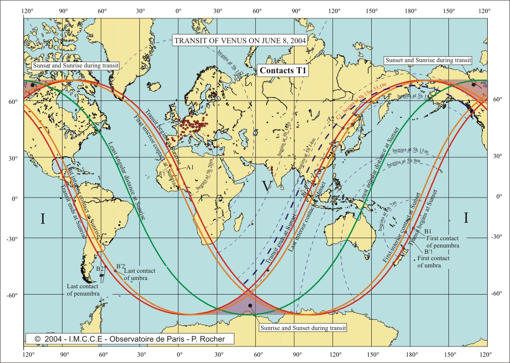
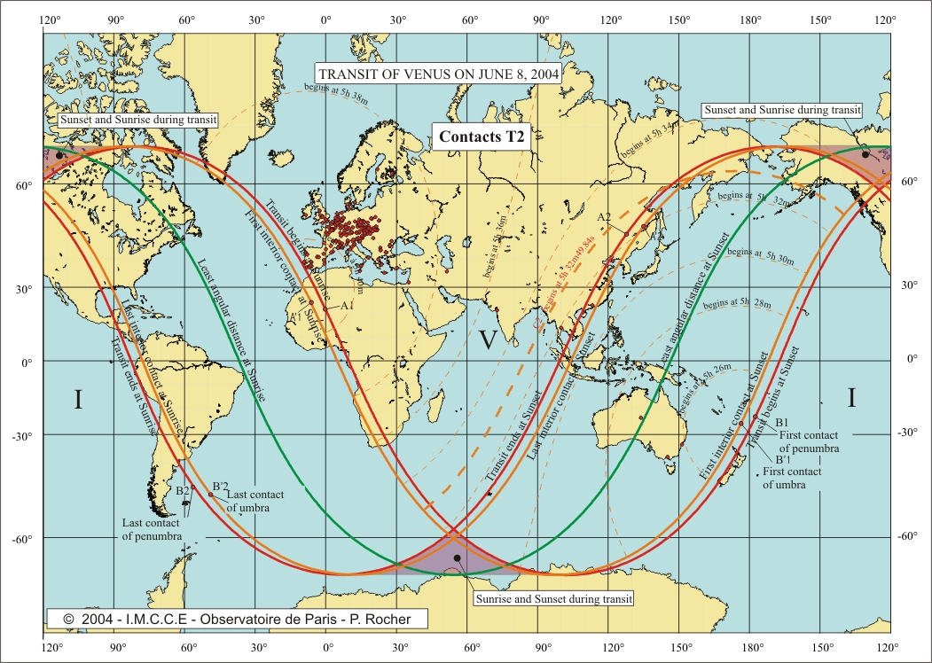
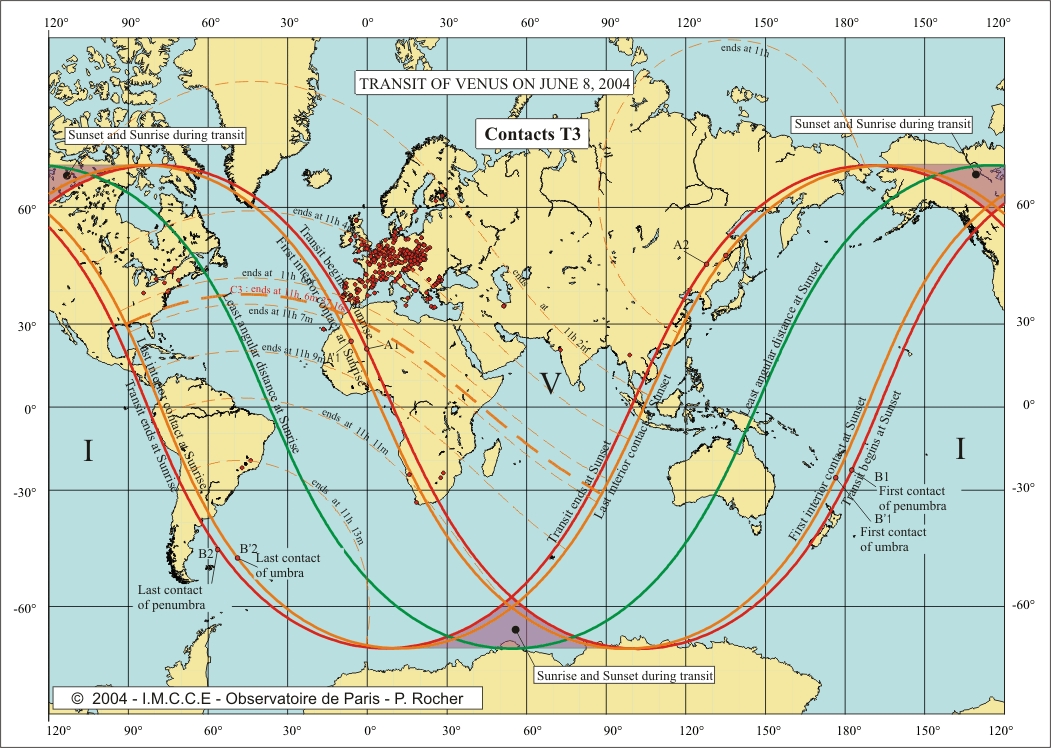
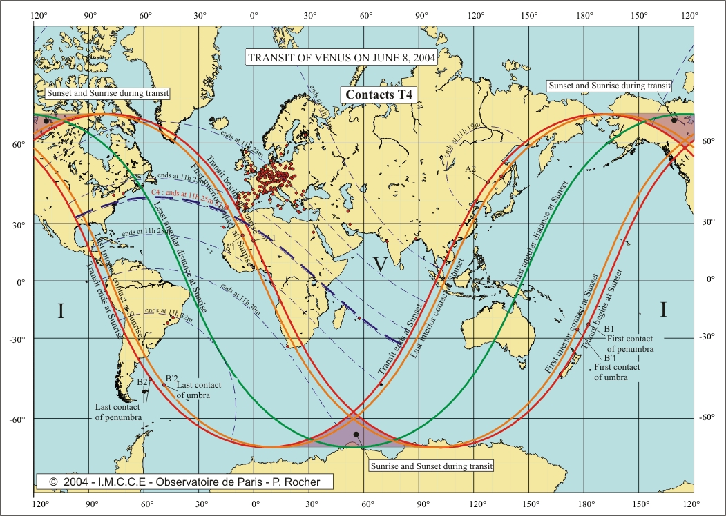
The four maps at the end of this note provide, for each contact, the curves corresponding to a contact at a given instant t. We plotted in bold the curves C₁, C₂, C₃ et C₄ corresponding to the sites on Earth observing the contacts at the same time than the centre of the Earth. We also plotted on these maps the observing sites that we selected for our calculations and presenting a difference less than 8 secondes with the predictions (interval 2DT = 16s).

Certainly the method of Delisle is not very powerful from a statistical point of view, but it keeps all its teaching interest. We thus extracted from the whole set of data, a data base formed by the "good observations". On this data base, students and pupils will be able to use the method of Delisle on two observations of their choice and to realize thus that all the sites of observation are not equivalent, even with equal measuring accuracies.

In conclusion :

In conclusion, our best result on the AU is obtained by the linearization method (not constrained system) using the timings within 4 seconds of time (interval of 8s) from the prediction:

AU = 149 608 708 km +/- 11 835 km (diff. to AU 10 838 km)

for the system not constrained (583 observations in a interval of 8s)

UA= 149 840 958 km +/- 310 577 km (diff. to AU 243 088 km)

for Delisle’s method with all contacts (4386 combinations from 1066 observations in an interval of 16s).

The result obtained by the linearization method is better than the one obtained in real time since we eliminated the bad observations and better than the one obtained with Delisle’s method since the observing site were not well distributed on Earth. Note the elimination of more observations (observations within 3 or 2 seconds of time) does not provide better results (too few data).